MIAC compare the use of different house price simulation models for estimating losses from a typical lifetime mortgage (LTM) portfolio.
A key component of the simulation approach to LTM modelling is simulating house prices over the long-term future that follows the borrowers’ length of life, typically from age 55 to the maximum age in mortality tables which is around 120.
MIAC’s proprietary assets and liability management software Vision™ currently uses Geometric Brownian Motion (GBM) for simulating trending series, which includes house prices. We compare GBM against the more sophisticated ARIMA-GARCH (AutoRegressive Moving Average-Generalised AutoRegressive Conditional Heteroskedasticity) stochastic process in estimating house prices over the next 65 years, as there are well known limitations with the GBM process. Some of these are outlined below, and have the potential to be remedied by using an alternative approach like the ARIMA-GARCH process.
- ARIMA models score higher than GBM both in terms of point forecast and distribution forecast accuracy
- Serial autocorrelation is required to capture prolonged negative house price changes to simulate potential downturns in the index
- The geometric BM is a Markov process; the probability distribution for the next time step only depends on the current state. The history is discarded whereas house prices show autocorrelation
- Volatility in asset prices will not be constant over time, as is the assumption with GBM. In an ARIMA-GARCH process, the error or shock terms are scaled by the variance term σ 2t , in which a big movement, is followed by another big movement in periods of clustering, known as ‘volatility clustering’ in financial time series
- Normality assumptions do not always fit the real-world data particularly in times of economic turmoil. This is why practitioners generally adjust the parameters when performing a calibration of GBM to historical house prices, particular the growth rate.
Approach
The GBM parameters are easier to ascertain in terms of the direct impact they have on the simulations,
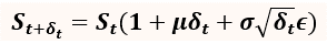
The drift term is the deterministic component, which reflects the longer-term trend in prices, is the volatility parameter, and the diffusion term √δ t ϵ is the stochastic component, reflecting shorter-term fluctuations. The noise term is a standard normal random variable,ϵ ~ N(0,1) .
We calibrate the GBM process to MIAC’s house price indices and use the projected house prices at the end of our 65-year forecast to determine parameter values for the ARIMA-GARCH model that would give a comparable house price distribution. This was achieved via a linearly constrained optimization.
The model specification for an ARIMA(p,q)-GARCH(p’,q’) process is as follows:
An ARIMA(p,q) model takes the following form
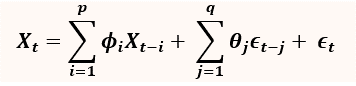
where ϵt=σt zt, Xt is the change in house price from time t-1 to time t, ϕi and θj are coefficients to be determined. The time-dependent variance σ t2 is approximated via a GARCH(p’,q’) model
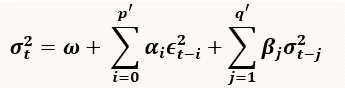
ARIMA(p,d,q) is the econometric specification which is comprised of: an autoregressive operator (AR) of order p, the dth difference and the moving average (MA) operator of order. The AR component specifies the number of historical lags that are used in predicting the current house price change Xt, the MA component incorporates present and past fluctuations and the dth difference represents the number of times the series was differenced to achieve de-trending. GARCH(p’,q’) models the volatility of the series using historical squared error terms ϵ 2(t-i) and volatilies σ2 (t-j) Hence the ARIMA-GARCH model possesses some memory and therefore serial autocorrelation.
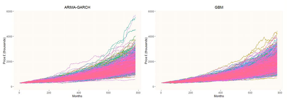
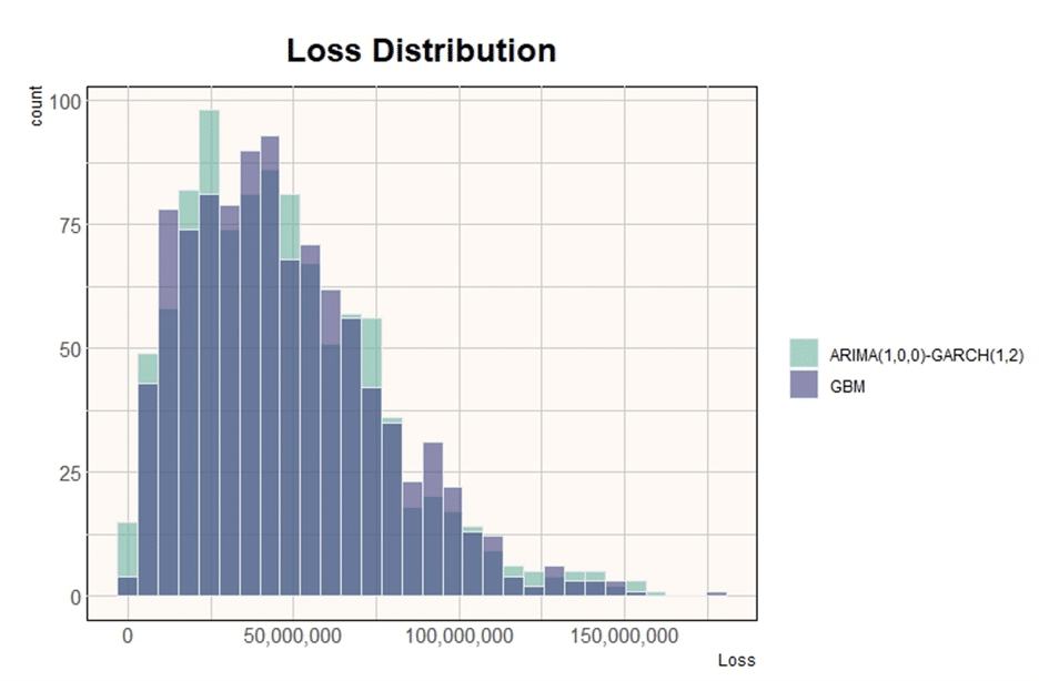
The following graphs show the simulated house price paths for both the ARIMA GARCH and GBM models over 65 years.
We derive dummy data for a typical LTM portfolio and simulate borrower exit events over the 65-year time horizon, where exit events correspond to either a mortality event or long-term care. Once an exit event is determined, the borrower’s property is liquidated, and loss is calculated by taking the difference between the property price and future balance. We simulate the lifetime portfolio for 1,000 borrowers, over 1,000 forward-looking house price scenarios, giving us 1,000,000 independent observations. Loss is summarised by aggregating over the simulations for all the loans.
Results
The loss distributions are very similar in shape, with losses concentrated at the beginning of the interval tapering off towards higher values, characteristic of a heavy right-skewed distribution. The ARIMA-GARCH shows a slightly higher standard deviation, and skewness relative to the GBM process, which is why we see a slightly higher 99th percentile loss calculated as a percentage of the balance.
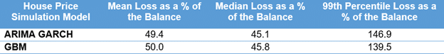
In conclusion the differences are not significant enough to justify trading the simplicity of GBM for the complexity of ARIMA GARCH type processes. In addition, whilst the ARIMA GARCH process does introduce the desired autocorrelation, we have not lost the normality assumption with the way we have implemented here. Our investigations did point to ARIMA GARCH being a far more accurate model with which to predict house prices which is something we continue to explore, however in calculating value at risk this is not necessarily the goal of the modelling exercise.
MIAC continue to investigate other simulation models for house prices and other macroeconomic variables for implementation within our assets and liability management system Vision™. For more information please get in touch www.miacanalytics.co.uk.